Field Activity #9: Surveying with a Topcon Total Station

Introduction

This activity was designed to further our surveying techniques by using a total station which captures z points (elevation) along with x and y.  Previous surveying techniques only gather X and Y points, however gathering elevations may be very useful and important in some cases.  This lab taught the class how to set up a total station, gather points using the device, and import the points on to ArcMap to view the results. 

Methods

The first step of the assignment was to learn how to set up the total station and collect points.  The total station was brought out to University of Wisconsin Eau-Claire's campus mall.  A 1 hector square was the goal to be surveyed around campus.  In figure 1 below the total station is placed on a tripod and pushed into the ground by stakes.  It is very important that the total station is level for surveying purposes.  The legs can be adjusted and levels are on the total station to see if it is even.  

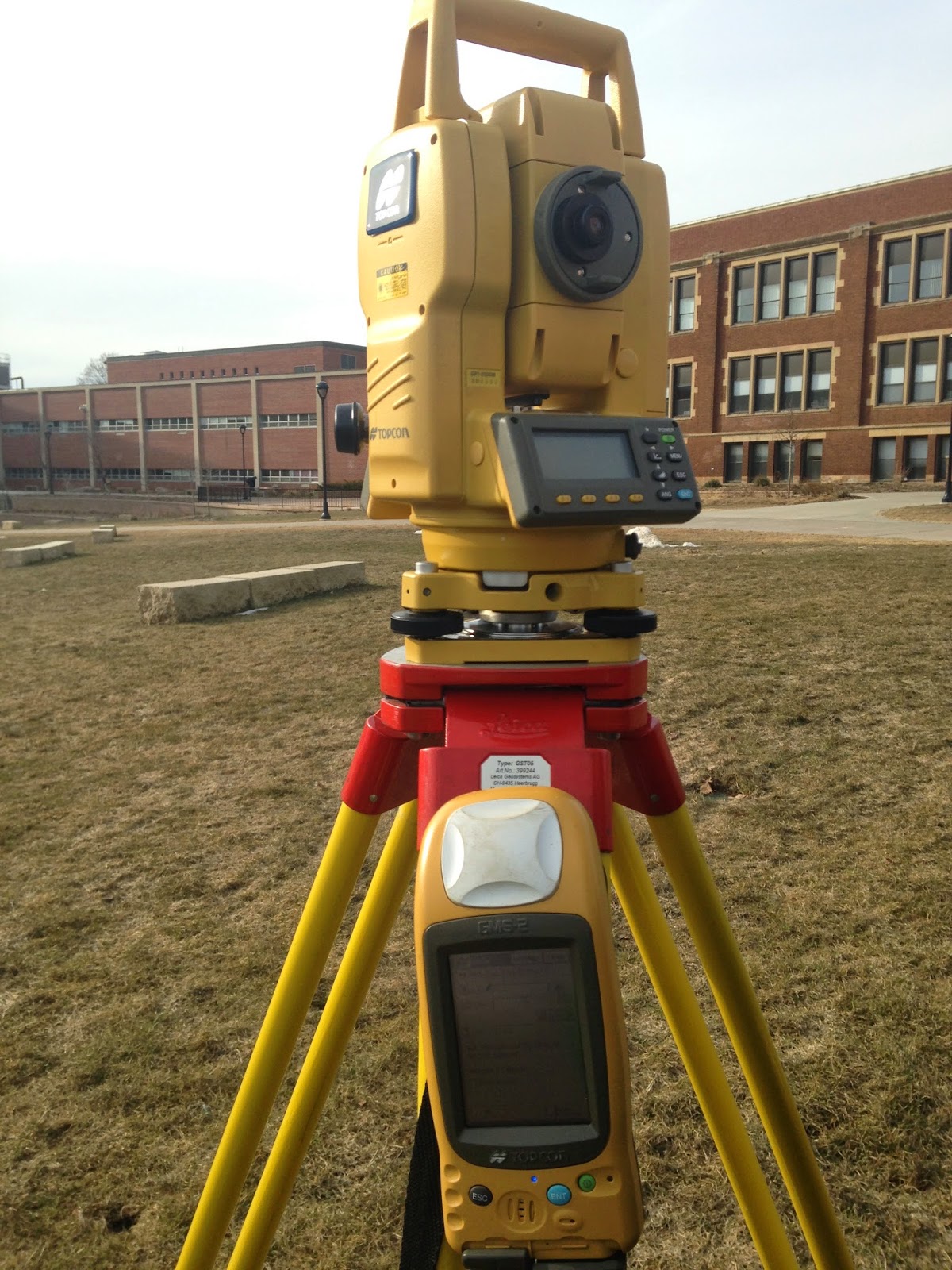
Figure 1: Total station set up on campus ready to be used to survey. 

There are also three black circle nobs that are used to raise the total station to help make it level.  Once the tripod is level it is ready to be blue toothed to the GPS unit (seen in figure one resting on the side).  The GPS unit also has to be set up ready to be surveyed by collecting a back sight and OCC point.   To blue tooth both instruments first it has to be turned on, found in parameters on the total station.  Once the blue tooth is turned on it can be connected on the GPS unit.

In the GPS unit data collection was chosen to start the set up of collecting.  First a new job was created. In here the setting can be modified to fit the specific needs of the collection.  Group one was entered for the name of the new job.  The coordinate system "UTM Zone 15 north NAD 83 was chosen because Eau Claire falls under that zone.  Meters was selected for distance, Gird for coordinate type and other settings were selected a step by step can be seen below created by Joe Hupy our professor.  

    1.      Set up Blue Tooth

a.      Turn on the total station.

b. Turn on the station Bluetooth. This is done within the menu area, and within the parameters portion. 

c.       At this point, you will not see a Bluetooth symbol appear on the TSS. This will appear after you set up the TopSurv Job.

    2.      Set up TopSurv Job

a.      Set up TopSurv Open up TopSurv (if no short cut appears find the EXE in the Flash Disk by clicking on My Device from the home screen, then flash disk, and then TTS folder)

b.      If TopSurv has icons instead of menus click the Topcon Icon in the upper left corner and Switch Menus

c.       Inside TTS  - Make a new job

                                                              i.      The open job menu will appear

                                                            ii.      To make a new job click new

                                                          iii.      To type in a name click on the space and a keypad will open up

                                                           iv.      Click next choose My RT DGPS for GPS + Config and My Reflectorless for TS config.

                                                             v.      Set the projection accordingly.

1.      If you are planning to enter the coordinates in manually from a different GPS unit you need to choose the same projection as the coordinates that you have from the other unit.

                                                           vi.      You may also need to change the datum (ex if you are using UTM N 15 NAD 83).

                                                         vii.      Do NOT check grid to ground

                                                       viii.      Set the Geoid to the first one that is in the list.  Click next.

                                                           ix.      In the units menu set your distance units to meters and choose whatever else you want for temp etc.

                                                             x.      Coordinate type will be Grid, coordinate order should be Easting, Northing, Ell Ht. leave the rest.

                                                           xi.      Turn on alarms if you wish.

                                                         xii.      Finish

d.      The blue tooth manager will appear. Select the GPT (TSS) then choose select. It should connect to the GPT. The blue tooth light on the GMS-2 should be blue indicating that it is connected.

e.      You may need to go to the Job Menu, and go to Observation mode. Select Total Station. You could select GPS if you were using the GPS + a LAZER.

f.        If a window pops up asking you for codes

                                                              i.      Type in the following codes for

1.      The key value should read  2951612344

2.      TS: 142601006

3.      GIS: 142601214

After following these steps to set up the job the next step is to collect a back sight point and the OCC point.  The OCC point is to let know the device where they are located in with a lat and long coordinate.  After collecting the OCC a back sight needs to be created.  A back sight is used to let the total station know where north, south, east, and west are located.  Without a back sight the collected points would be floating somewhere in space.  After collecting the back sight the total station can now use that point in reference to all the other points collected.  To do this follow these steps below:

    1.      Collect GPS points with the GMS2 in TopSurv*

a.      From the Job menu, go to Obs mode

                                                              i.      Check GPS+

b.      Then go to collect menu, and collect features

c.       The point will auto label OOC1 – keep tract of  this as you will need the name again

d.      Place the GMS2-s over the laser point for the OCC. and click start. The GMS2 will begin logging points.

e.      If the GMS-2 will not log points, click on the settings button and the top and choose solution type DGPS, Auto. You can also set the number of positions to be averaged. This can also be set from the job configuration menu.

f.        Once you have collected enough points for a position for the OCC you can click accept.

If you wish to also record the location of the BS at this time you can follow the same procedure.

*Both the occupied point and the Back Sigh (BS) are as accurate as the GPS unit you are using. If you wish to attain higher accuracy, it is recommended that you use a separate GPS unit that averages a high amount of points as the information you enter

     2.      To begin the OCC/BS setup

a.      Go back to the job menu, observation mode, and choose Total Station. Then proceed with Step 8 (skip step 7)

     3.      If you have X,Y coordinates from a different GPS unit and you wish to add the OCC/BS points in manually then:

a.      From the edit menu go to points.

b.      Click on Add

c.       Then click on New

d.      Name your point accordingly (ex. OCC1). Type in the coordinates you obtained from the GPS unit.  These MUST be in the same coordinate system AND Datum as the settings from the GPS unit.

e.      Click finish.

f.        Repeat for the BS.

     4.      Set the OCC and BS.

a.      Go to the Col menu, choose OCC/BS setup.

b.      If OCC/BS does not appear in the menu check the File menu, Observation Mode and be sure it is set to Total Station.

c.       In the BS setup tab, in OCC spot click, on the drop down menu to the far right and choose from list the point for the OCC (either that you collected with the GMS2 step 6 or added manually step 7).

d.      Choose the point where the TSS is located – the OCC point you entered in the previous steps

e.      Then set the height of the instrument by measuring the to the mark on the TSS from the ground up

f.        Then set the height of the prism from the rod

g.      If you wish to enter the BS point from the list

                                                              i.      Then be sure the button next to the pointing figure says BS Point, if it says BS Azimuth click the button and it will change to BS point.

h.      Use the pull down menu to find the BS GPS point (same way you did with OCC). Select that point.

i.        Then sight the TSS to the BS. You do not need the prism on the BS you just need to have the TSS sighted in the exact direction of the BS.

                                                              i.      FYI if you want to put the prism on the BS – no harm will be done

                                                            ii.      FYI if measure dist to BS is checked then the prism must be at the BS and the TSS will shoot the BS.

j.        Once the TSS is sighted to the direction of the BS then click HC set. The BS Azimuth will then be set to zero even though it is not north. This is OK because the software/TSS automatically does the calculations. This is so everything is relative to the angle between those two points.

k.      If you wish to use BS Azimuth

                                                              i.      Orient the total station in the EXACT direction of the BS and enter in the angle from north for the BS. You can use a compass or laser find to measure this angle. The follow step j above.

l.        You are now actually ready to collect data.

After the the OCC and Back sight are collected the collection is ready to be started.  In this survey a topographic survey of campus mall was done.  A total of 109 points were collected by our team around an hour.  To collect the points the total station uses a laser to find the prism pole, figure 2, one of our groups members was holding out in the field.  

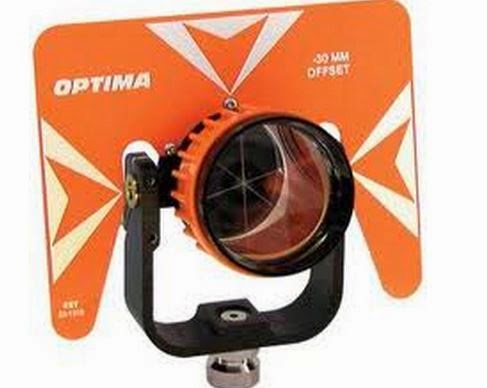
Figure 2: Photo of a prism, similar to the one used for the collection. 

To survey one person needs to be at the total station looking through the total station lenses and finding the mirror on the prism.  The total station then uses the laser to locate the prism in terms of X,Y, and Z coordinates.  When holding the prism in the field it is important to keep it as straight as possible and collect an array of points.  If an area is relatively flat it is not needed to collect a lot of points in the area because the elevation does not change.  However, when the elevation does change drastically in an area a lot of points need to be taken to cover the elevation change.  In our data collection the land was relatively flat except for the area down by the river.  However, a lot of points were collected for practice.  

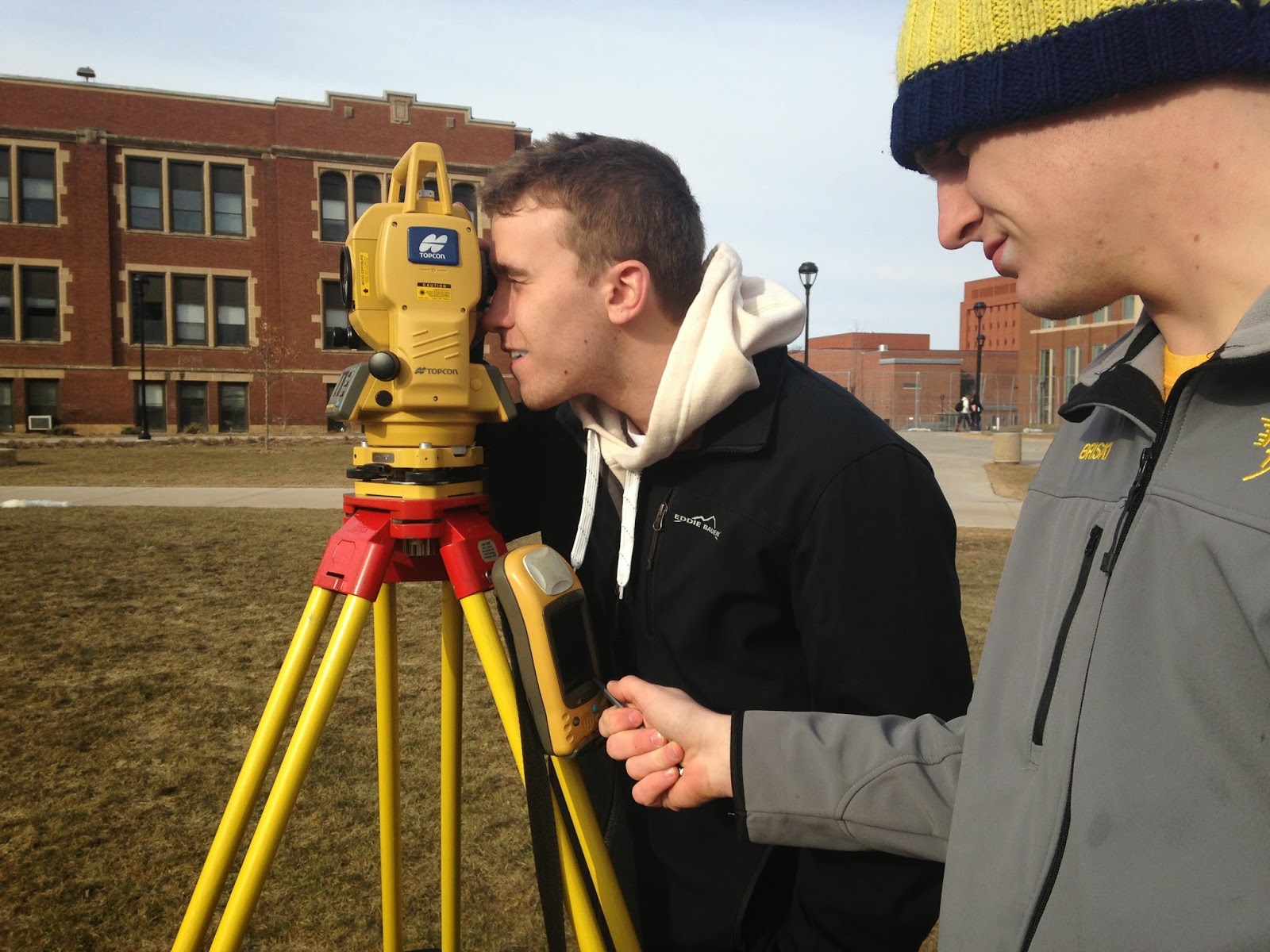
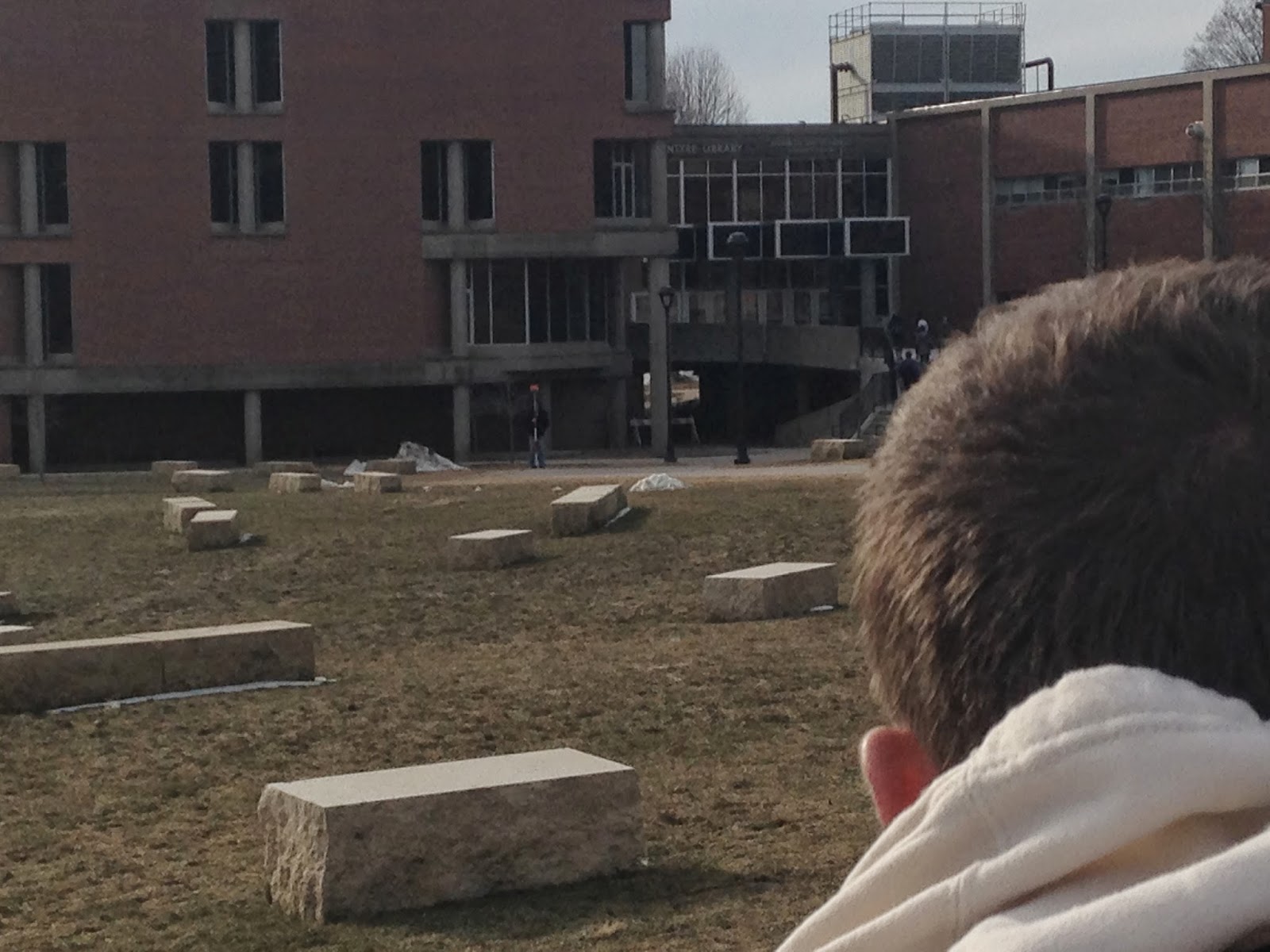
Figure 3: Image of me looking through the total station lens trying the find the prism.
Drew is ready to hit the collect button on the GPS once the total station and prism are matched.  

Figure 4: Image of me finding Andrew holding up the prism.  As you can see
he is about 50 meters away wearing a black shirt.  The total station has very
good optics so finding someone at a distance is easy.  

     1.      Collect Data

a.      Go to the Col menu and choose observations.

b.      Then click measure once the TSS is sighted to the prism. Continue to do this and make sure that the point’s id numbers are increasing.

c.       If you wish to verify the data, go to edit and list and look at the points you collected. You can also view these points on the map tab

d.      Continue collecting data.

e.      Be sure that if you change the height of the rod you must enter the new height of the rod into the collection screen for each point. 

After the collection is over the next step is to add the data onto ArcMap.  One problem that occured when bring the points into ArcMap was that they were flipped.  To unflip them the rotate tool was used so the points were in their correct positions.  

Results

The results of our surveying turned out well.  The amount of points that were collected worked out and gave us a good read of the elevation on campus.  However, I wish we would have surveyed more points down by the river to really see the elevation change down there.  The land surveyed was relatively flat making it easy to survey and the results don't look as cool when the land is flat.  

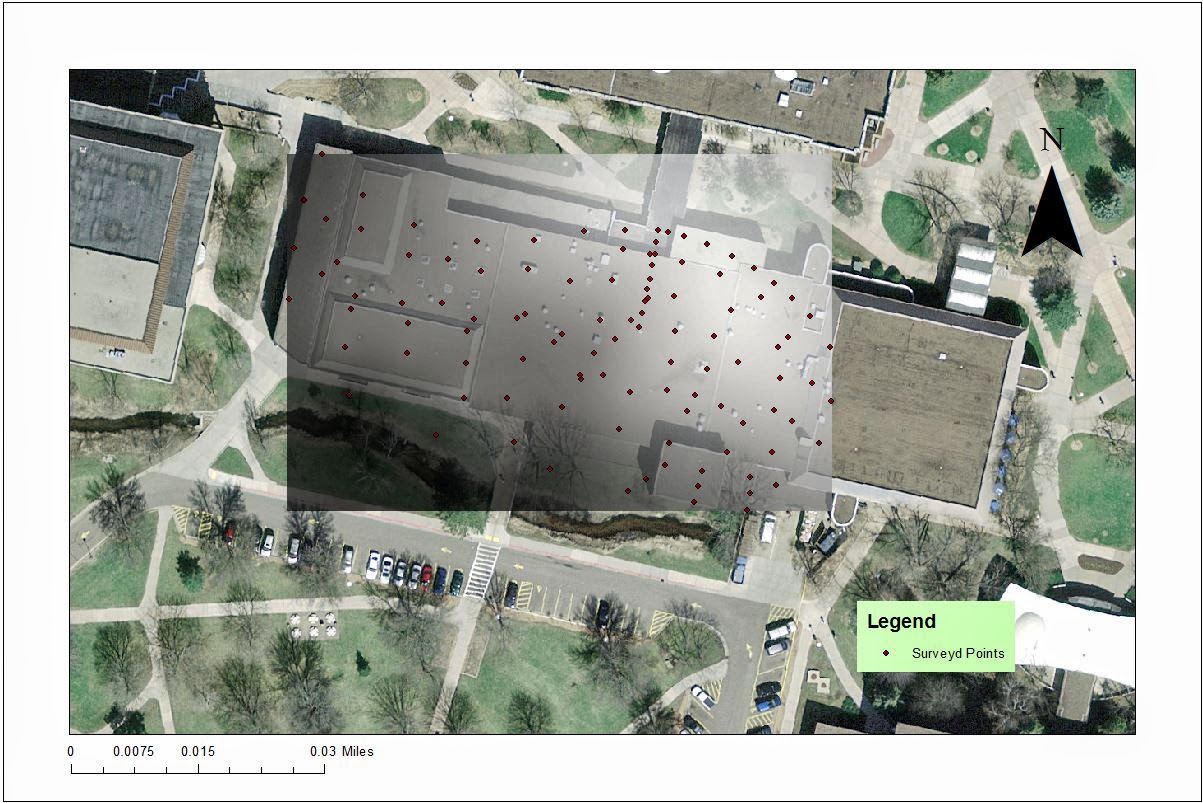
Figure 5: 2D result captured on an aerial image.  I could not find an updated image as
the building on our points does not exist anymore.
The black represents low elevation while the white is high

Figure 6: This is also an image of the points collected using ArcScene.
Natural neighbor was applied to the points resulting in the white being high elevation
and the green being low.  

Because of the area we surveyed and the elevation not changing much it was hard to get a 3D picture of the elevation.  When using an interpolation method in ArcScene the result would be flat, there for not being able to see a change in elevation.  

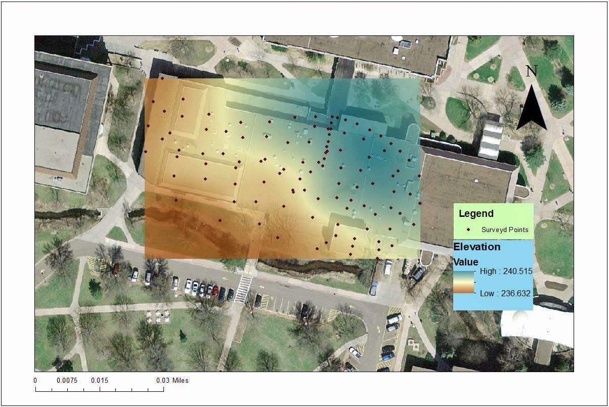
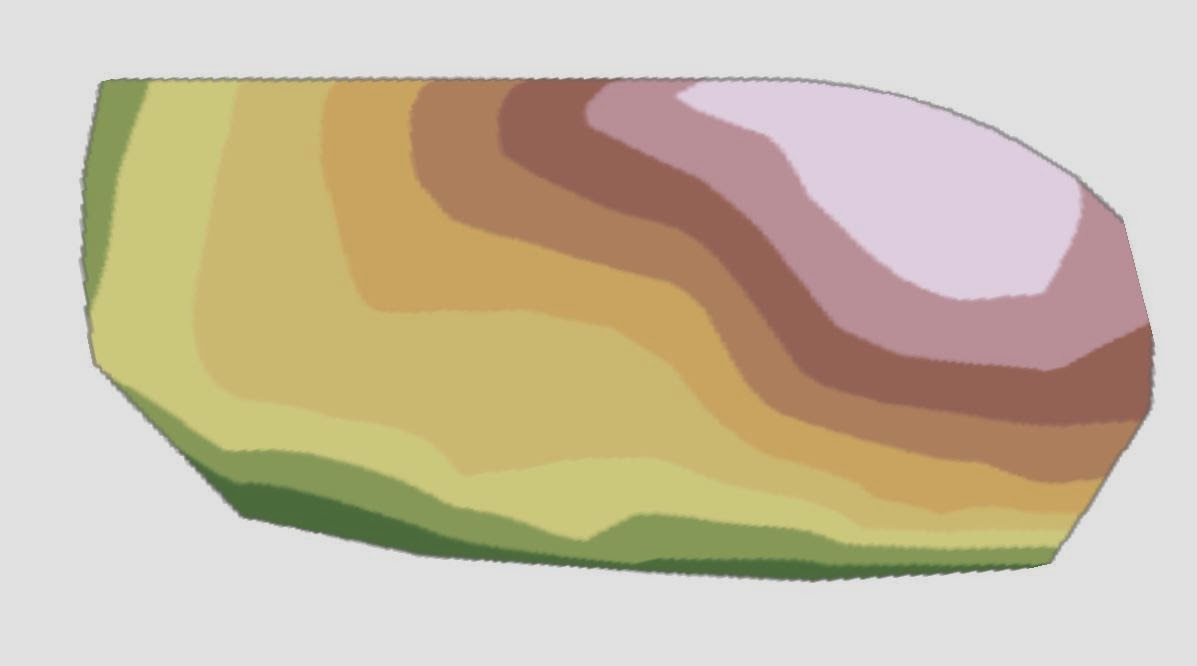
Figure 7: A final cleaner map of the points collected.  This color scheme makes it easier to read where the
low and high elevations are.

Conclusion

My group worked very well together when collecting the data.  The collection went fairly quick as I have had experience with a total station before allowing me to find the prism at a quick rate.  We had trouble setting up the GPS with switching modes to be able to collect the back sight and OCC point.  Once that was taken care of it was easy rider after that.  I would have liked to survey a place that had a greater change in elevation for a better looking 3D map and better practice when collecting an area with great elevation change.  

Field Activity #8: ArcPad Data Collection

Introduction

This weeks activity involved gathering micro climate data using a Trimble GPS unit and temperature gauge, then mapping the information by using ArcMap.  The class was divided into groups of two and the task was to gather points in an area on the campus of University of Wisconsin Eau-Claire.  The activity called for collecting temperature, dew point, relative humidity, snow depth, wind direction, as North, South, East and West, and also azimuth 0-360 degrees, wind speed, time, and any notes to help better the collection.  After all the groups collected data for their area the points were compiled into one geodatabase ready to be used to map out the results.  

Methods

The first step of this activity is getting the GPS unit and ArcMap ready for the collection.  Two weeks ago, see field activity #6 blog, a domain was created for this assignment and was placed, along with a raster image of UWEC's campus into ArcMap.  To load the domain, or feature class, and raster image on to the GPS or ArcPad these steps need to be taken.  In ArcMap click on customize>extensions> and check ArcPad Data Manager, this will allow you to use that tool.  Next add the toolbar to ArcMap by clicking Customize>Tool bars> ArcPad Data Manager.  Then click the first button as figure 1 displays to start adding the data to the trimble unit.  

Figure 1: Click on Get Data for ArcPad

After clicking this button a box will appear and click next from the welcome screen.  Hit the action menu and choose all Geodatabase layers, and also click on the raster image and click export as background TIFF.  Then in the next screen under specify a name type 'micro_yourusername' this will create a folder for all the information.  Also change the path of where the file is stored by clicking on the little folder and put in the folder you wish to store the ArcPad data information.  Then in the next window click on create the ArcPad data on this computer and finish.  Once the project is created, copy the folder and paste it for backup in case there is an error in the process or out on the field.  

The next step is to put the new feature class and tiff image onto the ArcPad GPS unit.  Connect the trimble unit with a USB port, and once the Trimble unit is in the computer and files can be viewed copy and past the newly created folder into the storage card of the Trimble unit.  After this is done disconnect the trimble and click the button top right corner labeled ArcPad 10 as you can see in figure 2 below.  Next hit open new map and choose the new folder that created for this process, figure 3.

Figure 2: ArcPad 10

Figure 3: Choose new map to open

After these steps and with the raster image loaded to the device you are ready to go out into the field and collect data.  Using the Trimble GPS unit, figure 4, a compass, meter stick, and the Kestral device collecting the data should run quite smooth.

Figure 4: Trimble GPS unit.  When first turning on the trimble make sure the GPS is getting a signal or fix,
to allow for the GPS to know your exact location of the points created. 

Figure 5: Kestrel device, can read temperature, dew point, relative humidity, and wind speed.  

Once out in the field and in the study you and a partner can work as a team to collect the data quickly.  In trimble unit find the green circle button that collects a point and allows you to enter the information for temp, dew point, wind speed, etc.  Use the meter stick to measure snow depth, compass to find the wind azimuth and direction and the arrows on the kestrel unit will allow to move across the different elements of temperature.  Once collecting all the information move onto the next point, since this is a micro-climate activity it is wise to collect points that are relatively close to each other, about 20 or 30 yards.  

Figure 6: My partner and I study area and the 23 points we collected.  As you can see we collected
points on the eastern side of campus.  After looking at the points collected
we could have done a better job at collecting more points to gather more information. 

Figure 7: Image of UWEC's campus and the class's study area.  A total
of 268 points were collected. 

After enough points are collected the next step is to take the trimble unit back to the computer and upload the points on to ArcMap.  This is done by going back to the ArcPad Data Manager and clicking on the fourth button 'get data from ArcPad.  In the box hit the green plus arrow navigate to the new folder with points and click import graphics or check in. After this is done the new feature class containing the points with the micro climate information will appear in the geodatabase created for this activity.  The next step is to merge all of the groups information into one feature class so the information can be mapped.  The step for this can be found in Tim Condon's blog, a classmates of mine, found here.  

The next step of the activity is to create a series of map's that display the information collected.  This was done by adding the merged feature class of the all the groups.  Then using the feature class's symbology to display different types of information.  To create continuous maps of temperature, dew point, snow depth, and relative humidity the arc tool box > 3D analyst tools and the interpolation technique of natural neighbors was used to map the data.  Also one of the assignments was to create a map that showed the wind speed and direction this was done in symbology> quantities> graduated colors> advanced> rotation and rotating it by wind direction azimuth.  An arrow symbol was used to show the direction of the wind as you can see in figure 8 below.  

Results

Figure 8: Map of Wind Speed and Direction, the wind were rather calm on this day only 3 reaching
over 10 mph, also the wind direction seemed to trend as a NW wind ,coming from, making the temps colder.

Figure 9: Relative Humidity Map, increased from west to east.  

Figure 10: Snow Depth Map of the Snow depths on campus in centimeters.  The snow levels
were rather low unless some snow was shoveled or plowed making the levels higher

Figure 11: Temperature map of Eau Claire, this is an interesting map as the
only real high temps came in one circle, it could have been a group error or located near a
heater. 

Figure 12: Temperature and Relative Humidity Map, there seems to be no trend
between relative humidity and temperature.  

Figure 13: Map of temperature and wind speed + direction.

This map shows that colder temperatures are associated with higher wind speeds, which makes sense.  However there is a wind speed of 10-11 in the warmest spot which is interesting to me.  It makes me believe that there was a heater or error by the group collecting the data.  

All of the maps do a good job of representing the data collected and some patterns can be seen.  There were some errors by group 3 and points had to be deleted between Murray and Towers Hall.  Somehow the points got placed near the equator which is very strange.  These points were deleted to make the interpolation techniques work.  

Conclusion

I thought this activity was very fun to complete.  I enjoyed making the maps to find the results of all data collected and I am very happy of how my maps turned out.  I wish I would know more about weather so I can make connections and see patterns more easily.  For example, the relationship between temperature, dew point, and relative humidity and how they effect each other.  In all it was a great learning experience for the class and a skill that is going to be very useful for the future.  

Field Activity #7: Introduction to UAV's

This week the class was introduced to different types of UAV's carrying cameras.  The goal of this week was to introduce and familiarize the class with using different types of UAV's to capture images.  2 drones, 1 kite, and 1 rocket were used to demonstrate how they work.  Dr. Hupy and his friend Max displayed their drones to class demonstrating how they fly and capture images.  Also Dr. Hupy used his personal touch by creating devices on a kite and rocket to capture aerial images.  Below will feature images of the different types of UAV's that were used to demonstrate to the class.

Figure 1: Dr. Hupy's drone next to the remote which controlled it.  This drone had a flight time of 15 minutes, meaning it could not travel to far away from the person controlling it. 

Figure 2: This is the camera attached to drone in figure 2, it was set to take pictures every 5 seconds.  The camera was placed on a device that keeps the camera always facing down and steady. 

Figure 3: Max is preparing to fly the first drone, roto copter.  Both drones are linked to a GPS.  The copter will automatically go back to the place it took off from if anything goes wrong.  This is very important in case the copter travels to far a way or there is a malfunction in the device.

Figure 4: This is an image of Max's drone which he created.  It uses six propellers compared to figure 1 having 3.  This drone also has a flight time of 15 minutes and is linked to a GPS.  This drone seemed to be more steady compared to the drone is figure 1, maybe because of the six propellers.

After both of the roto copters were brought into the air they had to be calibrated.  The calibration took about 3 minutes and is key into getting the copter to cooperate with the remote and fly straight and steady.

Figure 5: This is an image of the kite our class used to capture images.  The lines you can see coming off the string is a camera help up by a device that keeps the camera steady in the wind.  The kite is a less expensive way of capturing aerial images, however the wind needs to be in ideal conditions to be in use. 

Figure 6: Classmate, Blake is handling the kite with care letting it capture images every five seconds.  The camera can be set at any intervals, this day it was set to take a image every five seconds.

Figure 7: Two cameras were attached to this rocket which was launched into the air by an electrical circuit.  Only one of the engines was fired which cut out the flight time.  This technique was the least successful of three because of the short flight time and failure to launch properly.  This rocket was designed by Dr. Hupy and it will continue to be edited and made more efficient. 

Field Activity #6: Microclimate Geodatabase Construction for deployment to ArcPad

Part 1

This week in class we learned how to develop a geodatabase domain and then create a feature class out in our personal geodatabase later to be used next week when collecting data using a GPS. The task of the week was to decide what belongs in the feature class, creating the feature class, and then importing it along with a raster background image into ArcMap.  

The first step of the process was deciding what fields were going to be created inside the features class.  As a class we followed these questions to come up with our data: What is the purpose of the event?  What are you trying to examine?  What are the ranges you are going to be looking at?  What is the type of data you will be recording?  Pre-planning for what goes into a geodatabase when collecting data in a field is very important.  Because when out in the field you want to have everything set up perfectly to collect data.  For example when collecting a survey of temperature you could run into a technology problem.  If the GPS or temperature gage is failing it is important to enter into your notes field that problems occurred, therefore when looking back at the collected data it will be easy to remember what went wrong. Staying one step ahead when out in the field is critical in having a clean and efficient way of collecting data. More information of what to add to the geodatabase can be found here.

Next week the class will be collecting temperature data around University of Wisconsin Eau Claire's campus mall. Therefore the fields used in the collection will all relate to components of temperature.  The fields the class decided on were: temperature, wind speed, wind direction (azimuth in terms of degrees and direction; North, South etc), relative humidity, dew point, snow depth, time, group number, and notes.  All of these fields contribute to temperature and it is important to gather the data their information when displaying our results.  The wind speed and direction is critical to the temperature of the air.  Faster winder speed leads to colder temperatures and the direction of the wind will lead to warmer or colder coming into Eau Claire. If the wind is blowing to the south this means that the wind will be coming from Canada leading to colder temps in Eau Claire.  Also relative humidity and dew point are other important factors to the temperature.  If the air is very humid the air will be thicker and hotter compared to when the relative humidity being low the air will be thin and cooler.  Time will have also have a great effect on the temperature, the coldest temperatures of the day usually occur around 6 am and the warmest around 2 or 3 pm.  This will be important because groups may collect their data at different times of the day.   Snow depth was a personal choice for the class and does not relate the current temperate.  The notes field will be used to take any important notes during the collection.  Things like, "standing next to a building heater" or "the wind was blocked by buildings" will be important when reading the results of the data. 

 

Part 2

The next step after pre determine what will go into our personal geodatabase is to create the geodatabase.  To do this open up ArcCatalog and connect to the folder you wish to use when creating the goedatabase. To do this click the connect to folder button seen in figure 1.

 

Figure 1:The connect to folder button is shown in the image above.  It is the folder
with the plus sign in the corner.  This will let you connect to the folder you wish
to create the geodatabase in. 

 

Then after connecting to the folder desired, right click on it and choose new personal goedatabase.  This will create a geodatabse and the name of the geodatabase can be edited.

 



Figure 2: In ArcCatalog find the folder you wish to create the geodatabase and right click and
choose new personal geodatabse.  The new geodatabse should appear under the folder like
the image above shows the geodatabse mc_borgen_gdb

The next step is to edit the domain to set up the feature class.  This step is very important because you be setting the range of the domain along with the field type, short integer, float, or text.  Temperature, dew point, and relative humidity were set to float.  Notes and wind direction using north, south, east and west were set to text and the rest were set to short integers.  To see the domain right click on your personal geodatabase and click on properties and then domains.  Figure 3, should be seen on the screen and the domain is ready to be edited. 

Figure 3: When editing the domain this image should appear on the screen.
 You can set the domain name, field type, and range.

After editing the domain the next step is to create the feature class containing the different fields.  To do this right click on the geodatabase then followed by new and feature class.  The steps can be seen in figure 4 below.  Next set the class to a point feature class and choose a coordinate system seen in figure 5.  For this exercise UTM Zone 15N was used because Eau Claire fall within that zone.  More about UTM zones can be found here. 

Figure: 4: To create a feature class right click on your database followed by new and feature class.
The figure above should lead the way

Figure 5: For our study area the class used NAD1983 UTM Zone 15N.
The city of Eau Claire is falls in Zone 15.  

After choosing the coordinate system click next until you reach the image similar to figure 6.  Here you can edit the field name choose the data type and the domain type.  In the field name enter in each separate field, temp, dew point, wind speed, etc.  Then choose either float, short integer, or text for the data type and match it the domain entered earlier.  After entering the field name, data type, and matching it to the correct domain the feature class can be finished. 

Figure 6: An image similar to this should appear when creating a new feature class.
The field name, data type, and domain will have to be edited to create the feature class.

Also a background image should be imported into ArcMap for use when importing the collected data next week.  To do this follow the steps in figure 7 and import a raster image desired.   After the raster image is loaded into the geodatabase it, along with the feature class, is ready to imported into ArcMap.

Figure 7: Importing an raster image is rather simple, right click on the geodatabase,
then import, and raster datasets.  Then importing finding the raster desired
and placing it in the correct output folder it will appear in the geodatabase

To do this open ArcMap and click the add data button, which can be seen highlighted in figure 8.  Then connect to your geodatabase you created in ArcCatalog by clicking the connect to folder button seen earlier in figure 1.  Navigate your folder and add the feature class and raster image to ArcMap.

Figure 8: This figure is showing the box that appears when adding data.
The add data is the same button in figure 1, then by connecting the
folder containing the geodatabase add the data you want on your map.

If these steps are followed correctly your screen should be similar to figure 9 below.  The raster image appearing and the feature class and raster details appearing in the data frame.  You have now prepared a geodatabase with the correct fields ready to collect data and enter it on to ArcMap.

Figure 9: The image is the final result of creating the geodatabse, editing the domain,
creating the feature class, and adding the data to ArcMap.