Sunday, May 11, 2014

Field Activity #13: GPS Navigation Activity

Introduction

The final two activities are combined together because it was a two week process.  This activities involved  the class going back to the priory, see field activity #11 under study area, to navigate the entire 15 point course with a GPS.  The purpose of this activity was to create a map with of the points, a path, and the priory area to be downloaded onto the GPS to be used when navigating.  Again the class was split into groups of three and the goal was to finish the fastest.  This time the navigation came with a twist as paintball guns were provided for us to use and shoot opposing teams when they came close.  The paintball guns were provided by the geography department and Joe Hupy of the University of Wisconsin Eau-Claire. 

Methods

As I mentioned above the first week of the activity involved the groups to create a map of all 15 points to use on the GPS when navigating.  This is a very important step because without a clean map the naviagtion could become difficult when out in the woods.  The goal was to draw lines between each point to come up with the quickest path.  When choosing this path it was important to take into account of distance between points and elevation, figure 1 below, to find the fastest and easiest path.  

Figure 1: This is a map showing the elevations of the priory using contour lines.
We did not include the contour lines when uploading it the GPS because we thought it
would look really messy on a small screen. 
Above it can be seen that the highest elevation is located in the center of the map and the priory building at 310.  And the lowest point located at around 255 in the East and one in the West.  Our beginning point is highlighted in blue and we traveled northwest to our first point.  From there follow the black line as it loops entirely around the area and reaching the beginning blue dot. 

Seen below in figure 2, point 3 is located in a deep ravine so it was decided to knock that one out quickly so we would have a lot of energy to complete the rest of the course.  Points 6b to 2b are all located ontop of the hill, therefore staying up there was key when navigation to save time.  Then points 6a to 6 were located down the hill and back up again.  Our path utilized both the distance between points and elevation between the points trying to stay on lower ground and higher ground when possible, instead of running up and down the hill to save energy.  

Figure 2: Image of the points with labels to help show what I was describing above. 
After creating a path the final image, figure 3, was loaded onto the GPS to be used next week.  The purple areas indicate a no shooting zone because of the chance people not involved in the activity could be located there. 

Figure 3: The final map uploaded onto our GPS, we did not include the contour
elevating lines because we thought it was look clustered on a small
GPS screen. 
The navigation itself was rather easy using the GPS.  Our group would look at the GPS and follow the line until we saw the flag marking the point.  The hard part of the activity was carrying the paint ball gun and watching for opposing teams.  Drew was holding using the GPS and collecting a marker at each point, while Andrew and I would keep guard in case any one was close.  The rules with the paint ball gun were simple; if anyone in your group was shot you must stop moving and wait a 1 minute until proceeding again.  This would slow the navigation down and cost a team vital time.  The other tricky part of the exercise was being paranoid of other groups and becoming very hot because of the heavy and thick clothing that is usually worn during paintball.  During the end of the navigation our group constantly had to stop, remove our masks, and take a breather to cool off.  Even with all these factors our group managed to not get hit with a paint ball and finish the activity 1st out of six groups. 

Discussion/Conclusion

Navigating through the woods is more difficult then I thought.  However, using a GPS rather than a compass and a map is much easier.  Simply by looking at a computer screen and walking towards a point can be easy.  However, I would highly recommend becoming familiar with the map and where you are in relation to it.  If this would have been the first time our class would have been in the woods around the priory this activity would have been much more difficult.  Invloving paint ball guns was a brilliant idea.  It made me think I was apart of a mission team, and our goal was to reach an objective with out being seen or shot.  As a guy that lives to compete and finish first this activity was a blast.  However, I wish we would have ran into opposing teams more often for a mini battle to occur but, because of the larger area and thickness of the woods seeing other teams was uncommon. 


Saturday, May 10, 2014

Field Activity #12: Traditional Navigation Activity

Introduction

The purpose of this activity was to teach students how to navigate to different objectives using only a compass and a map.  This was done at the priory in Eau Claire, see study area below, and the goal was to navigate to 5 different points located in the woods.  The coordinates of the points were given before the activity started and by using the map and compass the objectives were marked on the map.  Using the points on the map and the compass the points were found in the woods using a very careful process.  The class was split into groups of 3, one controlling the compass, one counting using their pace, and one used as a marker to keep on the correct line.  

Study Area

Figure 1: This is a screen screen of the priory.  As you can see it is a very
'woodsy' area making the navigation at times somewhat difficult
The priory is owned by the University of Wisconsin Eau-Claire and has 112 acres of mostly wooded areas of land.  It is used for outdoor activities for students to learn and is also home to a children's center where students volunteer or work for educational experiences.

Methods
Learning how to use a compass to navigate on a map was done previously in the semester, and can be seen here for a recap.  Before we got started a geography student Zach Hilgendorf gave us a recap of how to use the compass when navigating.  The first step of the process was to map out the 5 points given to us by our professor.  The course was divided into 3 courses and each team was to navigate one course or 5 points.  Each x and y coordinates were given and by using the map created in field activity 5, the points were plotted (figure 2 below).

Figure 2: This is an image of our map used when navigating the course.
It is very hard to see but when looking close enough the black line can be
seen going from one dot to the next.  This represents the straight line
distance from one point to the other.  
After plotting each point the next step is to start navigating.  Each member of the group was given a job when navigating.  I had the job of using the compass to find the azimuth and straight line of where we should be going.  Andrew had the job of counting the pace between each point.  This job is very difficult because when counting your pass going up and down and over sticks in the woods it can be easy to lose track or count too high.  However, Andrew did an excellent job of navigating through the woods while keeping his pace.  Drew had the task of walking ahead of me and standing at a point of reference.  This step is very important when counting pace and navigating.  In the woods there is not a lot of room to see, therefore Drew would run up to a tree or a specific land mark where my compass was pointing too.  From there I would run walk towards him keeping my compass pointing in the right direction until I reached him.  Andrew would also use this as a tool when counting pace he would walk from me to Drew and just add the paces us at the end.  When I reached Drew we would start the process over ago from landmark to landmark until we reached the 5 points desired.  

Part of my job was to use the compass on the map and find the azimuth of where we were going next.  For example from points 1 to 2, I would place the compass facing 1 to 2 and line up with the north arrow.  From here the I would rotate the compass so it is directly facing north.  To do this you can align the compass with the grid on the map.  After it is facing north the azimuth is now found.  Then by keeping 'red in the shed' see figure 3 below, when walking the point can be found.  This is where Drew would come in handy, by keeping red in the shed I could walk towards Drew and keep a straight line.  I also could tell Drew where to stand by looking at where the arrow was pointing.  This step was done for all the points until they were reached and the marking was selecting at each point.  

Figure 3: when walking to the the desired point it is
important to keep 'red in the shed' seen above the red
arrow in the compass and also the red arrow on the compass,
when those two are lined up it is called 'red in the shed'

Figure 4: This is a photo of me, blue hat, figuring out the azimuth for the next point.
Finding the azimuth in the woods is difficult because it is hard to find a flat surface.
Andrew in the green shirt, is doing the math of his counted pace step.   
Figure 5: This is a photo of point 2, one of our objectives.
Navigating to this point was very difficult because it was
located in a deep ravine, climbing in an out while keep a
straight line or keeping pace was challenging.

Figure 6: This is an image of Andrew, green shirt, walking and counting pace
and Drew, blue shirt, standing at a tree for an landmark.  It is difficult to see Drew,
but by looking way in the distance you can see the color blue, or Drew. 

Discussion/Conclusion

Our group worked really well together by keeping the same job through out.  We found each point in a timely fashion and our navigation skills greatly improved. The most difficult thing about navigating was the terrain.  Walking through the thick woods with fallen over trees and branches in your way it became very difficult to walk in a straight line.  Also the elevation changes really wore our group down, if we were too do a longer activity it would have became more difficult.  The next activity will involve us using a GPS to navigate, this will be much easier but it will be nice to be familiar with the area.  


Friday, May 9, 2014

Field Activity #10 and #11: Aerial Mapping with a UAS

Introduction

Field activity's 10 and 11 were both combined together because they both dealt with Unmanned Aerial Systems.  Field activity 10 involved the class going out to our study area (see below) and capturing photos using a helium balloon that was raised hundreds of feet in the air.  The photos were then to put together a process called, image mosaic, using Photoscan.  The mosaic images were then georefrenced in ArcMap and placed on a map to see the results.  Field activity 11 involved our Professor, Dr. Joe Hupy, showing us the process of planning and flying a roto copter using a computer programmed to fly the copter, to capture images.  

Study Area

The study area chosen for these two activities was located at the Eau Claire Sports Center about 5 minutes from upper campus at the University of Wisconsin Eau-Claire. The reason we chose this area is because it is an open field soccer with not many trees or other features that might disrupt the UAS.  If the balloon or roto copter were to hit a tree it could damage it greatly and ruin the project.  

Figure 1: Image of the study area chosen by Joe Hupy, located
at the Eau Claire Sports Center

Methods

First I will explain with pictures the process Joe Hupy explained to us about planning and flying a roto copter because it does not involve as big a process as field activity 10.  

Figure 2: This is an image of the flight plan made by the computer program flying the roto copter
Seen above in figure 1 is a yellow line flying to 9 different checkpoints, the green dots.  After finding the study area on the program the checkpoints can be placed and the computer will run a flight plan finding the shortest distance to complete the point.  One thing Joe noted was to make sure to end the plan where it began other wise the roto copter will stay at the final point.  The copter flies around using a GPS it has installed to navigate through the area.  When flying the copter will collect images using a camera added to the copter.  Sometimes the GPS or roto copter will fail, therefore making it CRITICAL  to not perform this activity on your own.  If the roto copter gets destroyed that is valuable money being wasted.  Joe recommended one person at the computer controlling or monitoring the flight plan and the other watching the roto copter fly around to make sure no problems occur.  To see what the roto copter looks like, see my previous blog post field activity #7.

Figure 3: This is an image of the roto copter in the air, flying
around and capturing aerial photographs of the area desired.
The copter has an air time of about 15 minutes before it runs out of power.  

Figure 4: Here, our professor, Joe is describing where the copter is in
relation to the computer map.  The computer was placed on the garbage can
 in front of the study area to easily view the copter and computer. 


From here on out the process of capturing aerial images by a helium balloon will be explained followed by results and a conclusion. 

The first step of this activity was to fill up the balloon with helium so it can rise high in the air to take photographs.  The balloon is rather large, I would estimate about 10 feet high and very round.  After the balloon was filled the next step was to attach the handle and camera, seen in figure 5 and 6 below. 

Figure 5: What the man in the blue hat is holding is a device to lower or raise
the balloon, like you would use for a kite.  This is very important to focus on
as it controls the height of the balloon. 

Figure 6: Our professor, Joe Hupy, is attaching to cameras to the string of the
balloon with a device that keeps them flat.  The cameras were
 set to take pictures automatically every 5 seconds. 

After the camera was attached the balloon was lifted high into the air, figure 7, to let it capture aerial images.  The class took turns carrying the balloon, and it was made sure the entire area was captured.  

Figure 7: The balloon high in the air holding the cameras,
it was rather windy that day but the pictures turned out just fine.
It there would have been a little stronger wind the balloon might have failed.

Figure 8: The class walking on the edge of the field, one
person holding the balloon making sure the string does not hit a tree. 

After the entire field is captured the next step is to mosaic the images to create one clean image.  This is done with a program called Photoscan.  In Photoscan click on the Workflow tab and then Add Photos.  This will open up a new window will open and the aerial images can be added to the function.  After adding the photos, hit Workflow again and Align Photos.  This will run the photos for them to combined together but the picture will not be clear yet, seen figure 9 below.  Blake Johnson, a classmate, and I decided to work together to make our own mosaic.  We decided to only use around 40 photos to speed the process.  Drew Briski was the first one too run the system and his directions were followed precisely. 

Figure 9: Image of the photos aligned together, you can see the photos
lined up together but no real image yet. 

The next step is to build a mesh. Select Build Mesh under workflow.  This will create a TIN from the point cloud.  After the mesh was complete and the next step is to export the results as a TIN. Because the photos appeared darker than expected they were brought into Photoshop and the brightness values were played around with until the image desired was found. 

The next step is to export the photo as a TIFF so it can be georeferenced in ArcMap.  This is done by clicking File> Export Orthophoto>Export TIFF.  The below image of the Tiff can be seen if figure 10 below. 

Figure 10: The TIFF image created by Photoscan after the images
were mosaicked together. 
The final step to create the product desired is to georeference the image because the TIFF file is not correct and has no reference map or coordinate system.  The first step was to bring in the TIFF image and then the World Imagery from Arc Base Maps online.  Then zooming into the same area as the image so it can be referenced.   Georeferencing can be found by clicking: Customize> Toolbars> and Georeferencing.  Then in the Georeference tool bar click the viewer tool and bring in the tiff raster area of Eau Claire Sports Center.  Then click Add Control Points to start georeferencing the image.  To do this first find a location that can be found easily on both images and click there on the TIFF image first.  Then in the basemap find that exact same location.  Keep adding points first on the TIFF and then on the same exact location until the TIFF image is similar to the base map.  

Results

Below is the finished product lined up with surrounding features.  The image fits well in the base map except for the black edges around the image.  A total of 6 georeferencing points were added to both images to correct the TIFF file.   As you can see below the TIFF image is in black and white and somewhat blurry on the edges.  Maybe if more goereferencing points were too be added it would be fixed.  I am not sure how to fix the color though, that is how they resulted when using PhotoScan.  Drew Briski the master of the this assignment has a better outcome than me and his image is in color seen here. 

Figure 11: The final product from the balloon the ArcMap the photos are spatially
correct and match up with the surrounding features. 

Conclusion 

Capturing the aerial images from a balloon and then creating a TIFF is a long process.  It could have not been done with out our classmates Drew Briski and his knowledge with the PhotoScan program.  He set up directions of how to mosaic the images and create a TIFF file.  Without him this process could have not been done.  The result photo was decent, I would have liked it to be in color but I really have no idea how to change that because of my inexperience in PhotoScan.  


Sunday, April 13, 2014

Field Activity #9: Surveying with a Topcon Total Station

Introduction

This activity was designed to further our surveying techniques by using a total station which captures z points (elevation) along with x and y.  Previous surveying techniques only gather X and Y points, however gathering elevations may be very useful and important in some cases.  This lab taught the class how to set up a total station, gather points using the device, and import the points on to ArcMap to view the results. 

Methods

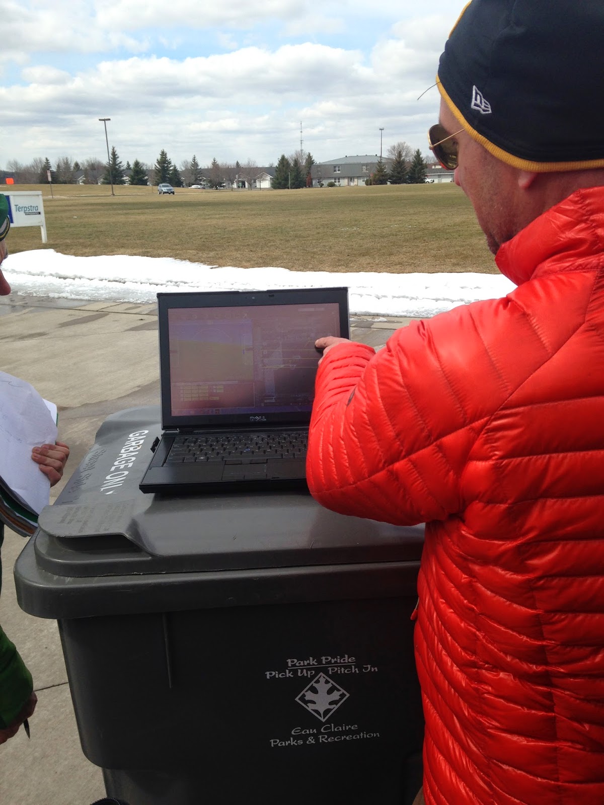
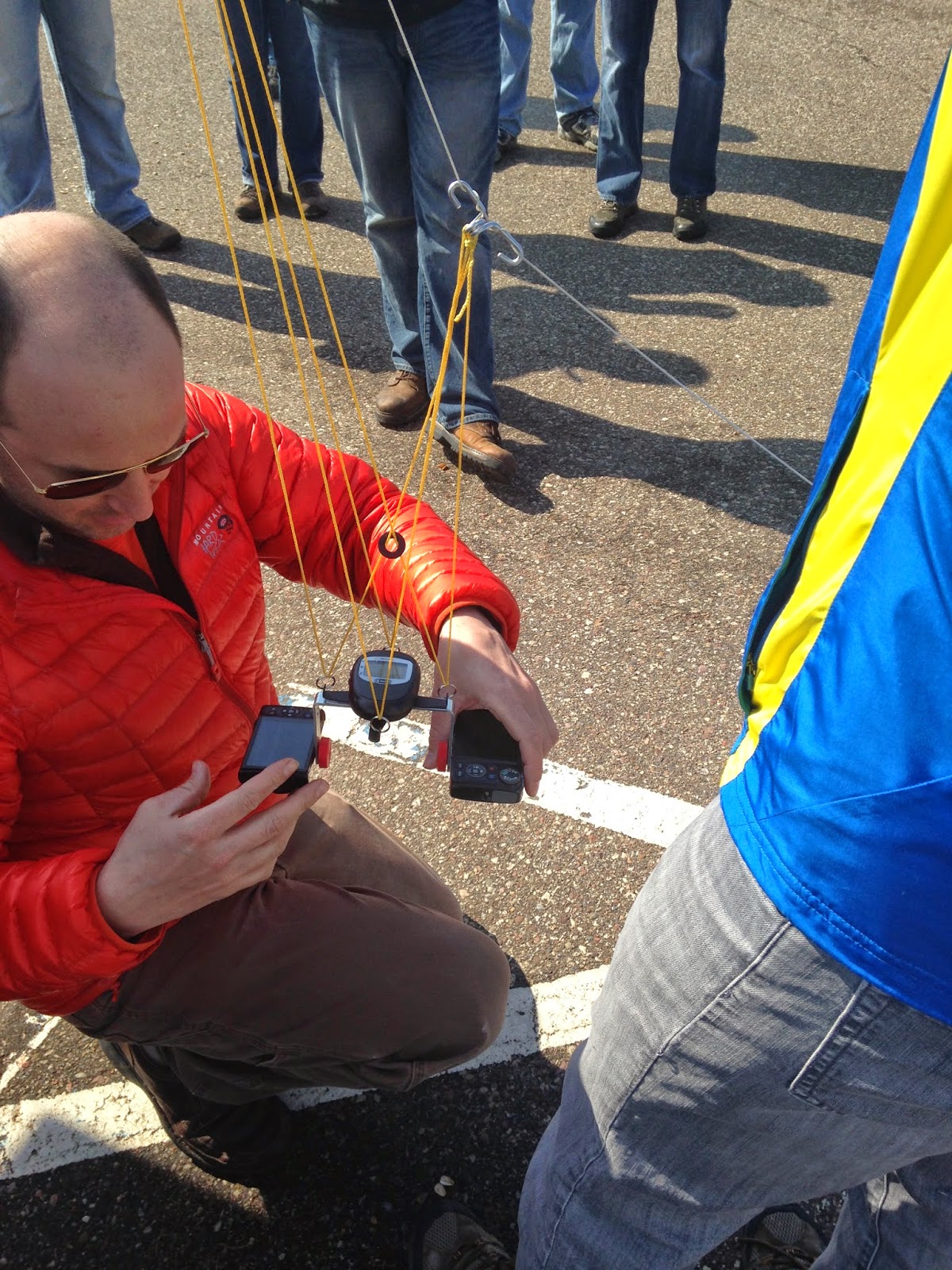
The first step of the assignment was to learn how to set up the total station and collect points.  The total station was brought out to University of Wisconsin Eau-Claire's campus mall.  A 1 hector square was the goal to be surveyed around campus.  In figure 1 below the total station is placed on a tripod and pushed into the ground by stakes.  It is very important that the total station is level for surveying purposes.  The legs can be adjusted and levels are on the total station to see if it is even.  

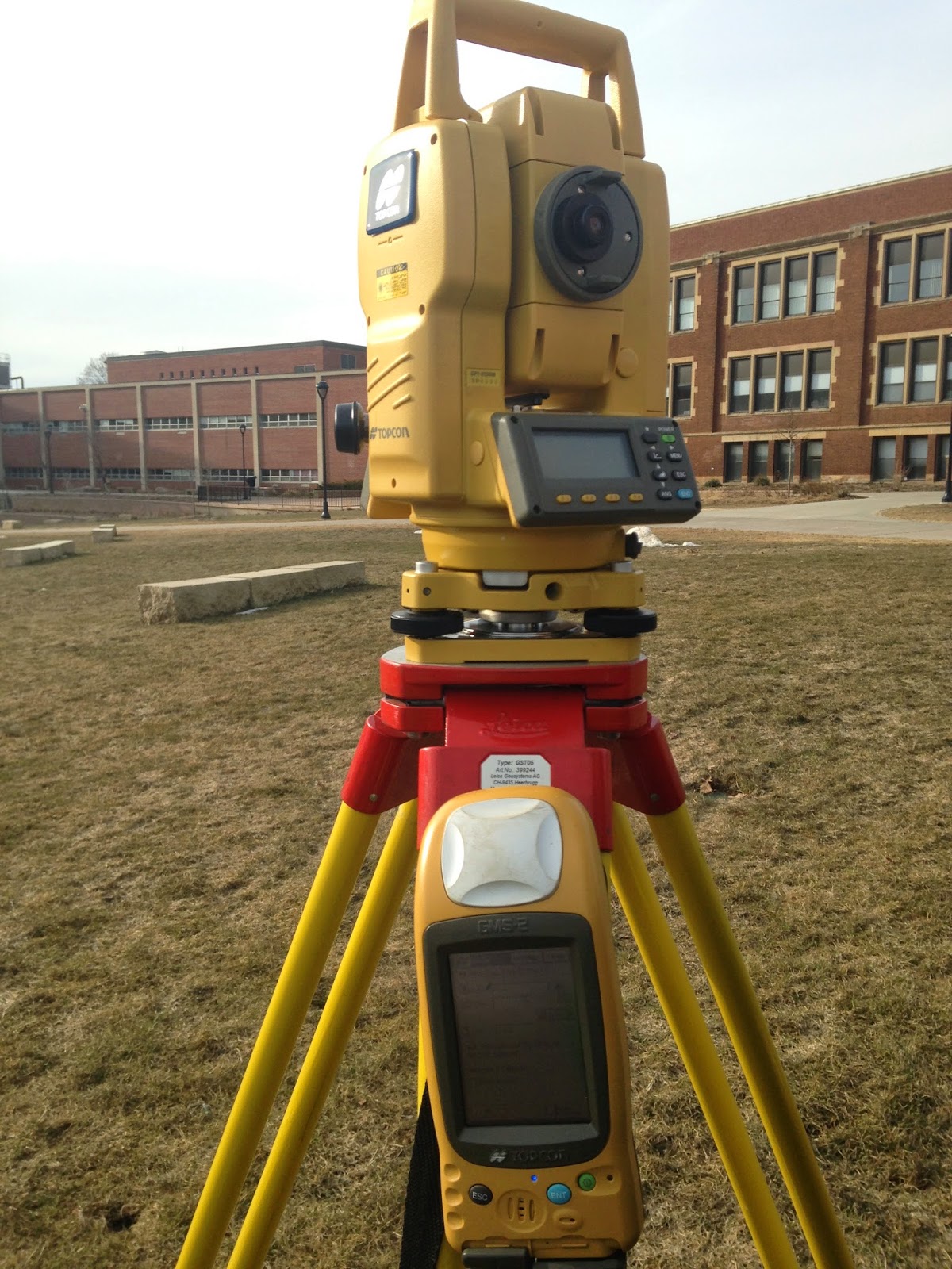
Figure 1: Total station set up on campus ready to be used to survey. 
There are also three black circle nobs that are used to raise the total station to help make it level.  Once the tripod is level it is ready to be blue toothed to the GPS unit (seen in figure one resting on the side).  The GPS unit also has to be set up ready to be surveyed by collecting a back sight and OCC point.   To blue tooth both instruments first it has to be turned on, found in parameters on the total station.  Once the blue tooth is turned on it can be connected on the GPS unit.

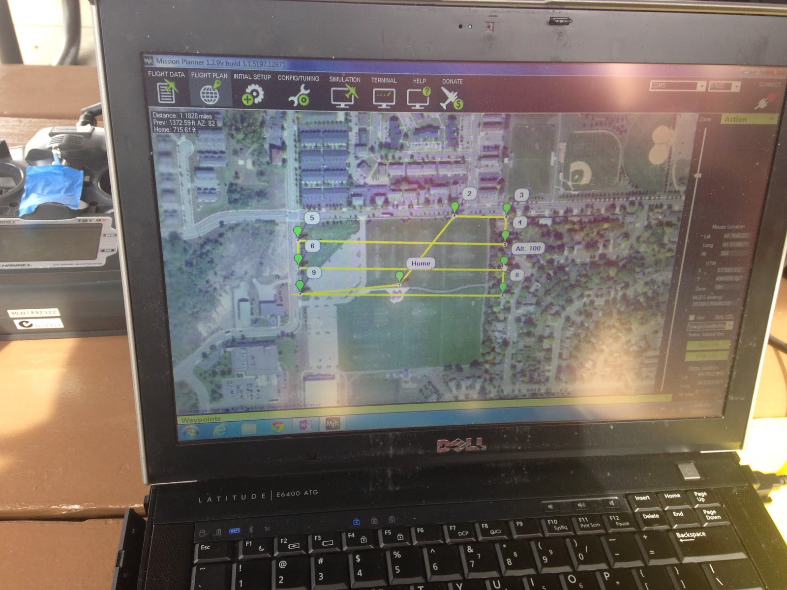
In the GPS unit data collection was chosen to start the set up of collecting.  First a new job was created. In here the setting can be modified to fit the specific needs of the collection.  Group one was entered for the name of the new job.  The coordinate system "UTM Zone 15 north NAD 83 was chosen because Eau Claire falls under that zone.  Meters was selected for distance, Gird for coordinate type and other settings were selected a step by step can be seen below created by Joe Hupy our professor.  

    1.      Set up Blue Tooth
a.      Turn on the total station.
b. Turn on the station Bluetooth. This is done within the menu area, and within the parameters portion. 
c.       At this point, you will not see a Bluetooth symbol appear on the TSS. This will appear after you set up the TopSurv Job.
    2.      Set up TopSurv Job
a.      Set up TopSurv Open up TopSurv (if no short cut appears find the EXE in the Flash Disk by clicking on My Device from the home screen, then flash disk, and then TTS folder)
b.      If TopSurv has icons instead of menus click the Topcon Icon in the upper left corner and Switch Menus
c.       Inside TTS  - Make a new job
                                                              i.      The open job menu will appear
                                                            ii.      To make a new job click new
                                                          iii.      To type in a name click on the space and a keypad will open up
                                                           iv.      Click next choose My RT DGPS for GPS + Config and My Reflectorless for TS config.
                                                             v.      Set the projection accordingly.
1.      If you are planning to enter the coordinates in manually from a different GPS unit you need to choose the same projection as the coordinates that you have from the other unit.
                                                           vi.      You may also need to change the datum (ex if you are using UTM N 15 NAD 83).
                                                         vii.      Do NOT check grid to ground
                                                       viii.      Set the Geoid to the first one that is in the list.  Click next.
                                                           ix.      In the units menu set your distance units to meters and choose whatever else you want for temp etc.
                                                             x.      Coordinate type will be Grid, coordinate order should be Easting, Northing, Ell Ht. leave the rest.
                                                           xi.      Turn on alarms if you wish.
                                                         xii.      Finish
d.      The blue tooth manager will appear. Select the GPT (TSS) then choose select. It should connect to the GPT. The blue tooth light on the GMS-2 should be blue indicating that it is connected.
e.      You may need to go to the Job Menu, and go to Observation mode. Select Total Station. You could select GPS if you were using the GPS + a LAZER.
f.        If a window pops up asking you for codes
                                                              i.      Type in the following codes for
1.      The key value should read  2951612344
2.      TS: 142601006
3.      GIS: 142601214

After following these steps to set up the job the next step is to collect a back sight point and the OCC point.  The OCC point is to let know the device where they are located in with a lat and long coordinate.  After collecting the OCC a back sight needs to be created.  A back sight is used to let the total station know where north, south, east, and west are located.  Without a back sight the collected points would be floating somewhere in space.  After collecting the back sight the total station can now use that point in reference to all the other points collected.  To do this follow these steps below:

    1.      Collect GPS points with the GMS2 in TopSurv*
a.      From the Job menu, go to Obs mode
                                                              i.      Check GPS+
b.      Then go to collect menu, and collect features
c.       The point will auto label OOC1 – keep tract of  this as you will need the name again
d.      Place the GMS2-s over the laser point for the OCC. and click start. The GMS2 will begin logging points.
e.      If the GMS-2 will not log points, click on the settings button and the top and choose solution type DGPS, Auto. You can also set the number of positions to be averaged. This can also be set from the job configuration menu.
f.        Once you have collected enough points for a position for the OCC you can click accept.
If you wish to also record the location of the BS at this time you can follow the same procedure.
*Both the occupied point and the Back Sigh (BS) are as accurate as the GPS unit you are using. If you wish to attain higher accuracy, it is recommended that you use a separate GPS unit that averages a high amount of points as the information you enter
     2.      To begin the OCC/BS setup
a.      Go back to the job menu, observation mode, and choose Total Station. Then proceed with Step 8 (skip step 7)
     3.      If you have X,Y coordinates from a different GPS unit and you wish to add the OCC/BS points in manually then:
a.      From the edit menu go to points.
b.      Click on Add
c.       Then click on New
d.      Name your point accordingly (ex. OCC1). Type in the coordinates you obtained from the GPS unit.  These MUST be in the same coordinate system AND Datum as the settings from the GPS unit.
e.      Click finish.
f.        Repeat for the BS.
     4.      Set the OCC and BS.
a.      Go to the Col menu, choose OCC/BS setup.
b.      If OCC/BS does not appear in the menu check the File menu, Observation Mode and be sure it is set to Total Station.
c.       In the BS setup tab, in OCC spot click, on the drop down menu to the far right and choose from list the point for the OCC (either that you collected with the GMS2 step 6 or added manually step 7).
d.      Choose the point where the TSS is located – the OCC point you entered in the previous steps
e.      Then set the height of the instrument by measuring the to the mark on the TSS from the ground up
f.        Then set the height of the prism from the rod
g.      If you wish to enter the BS point from the list
                                                              i.      Then be sure the button next to the pointing figure says BS Point, if it says BS Azimuth click the button and it will change to BS point.
h.      Use the pull down menu to find the BS GPS point (same way you did with OCC). Select that point.
i.        Then sight the TSS to the BS. You do not need the prism on the BS you just need to have the TSS sighted in the exact direction of the BS.
                                                              i.      FYI if you want to put the prism on the BS – no harm will be done
                                                            ii.      FYI if measure dist to BS is checked then the prism must be at the BS and the TSS will shoot the BS.
j.        Once the TSS is sighted to the direction of the BS then click HC set. The BS Azimuth will then be set to zero even though it is not north. This is OK because the software/TSS automatically does the calculations. This is so everything is relative to the angle between those two points.
k.      If you wish to use BS Azimuth
                                                              i.      Orient the total station in the EXACT direction of the BS and enter in the angle from north for the BS. You can use a compass or laser find to measure this angle. The follow step j above.

l.        You are now actually ready to collect data.

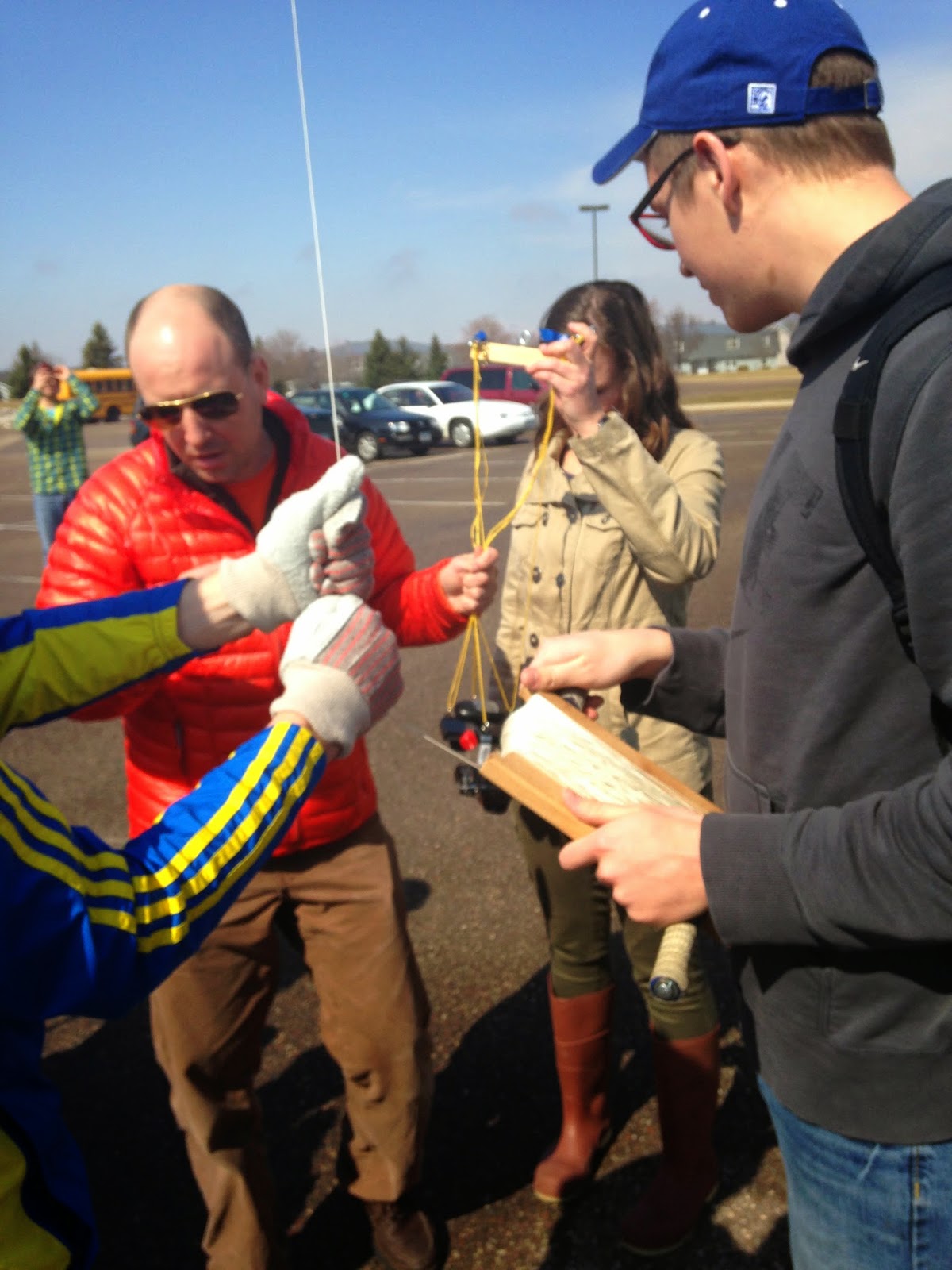
After the the OCC and Back sight are collected the collection is ready to be started.  In this survey a topographic survey of campus mall was done.  A total of 109 points were collected by our team around an hour.  To collect the points the total station uses a laser to find the prism pole, figure 2, one of our groups members was holding out in the field.  

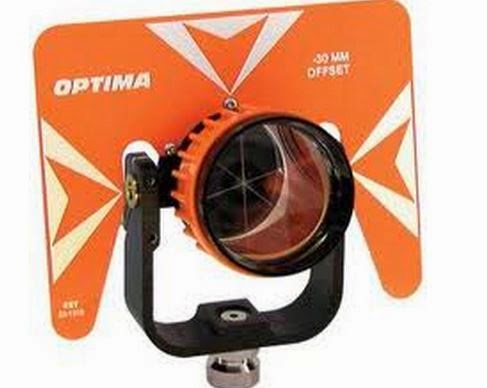
Figure 2: Photo of a prism, similar to the one used for the collection. 

To survey one person needs to be at the total station looking through the total station lenses and finding the mirror on the prism.  The total station then uses the laser to locate the prism in terms of X,Y, and Z coordinates.  When holding the prism in the field it is important to keep it as straight as possible and collect an array of points.  If an area is relatively flat it is not needed to collect a lot of points in the area because the elevation does not change.  However, when the elevation does change drastically in an area a lot of points need to be taken to cover the elevation change.  In our data collection the land was relatively flat except for the area down by the river.  However, a lot of points were collected for practice.  

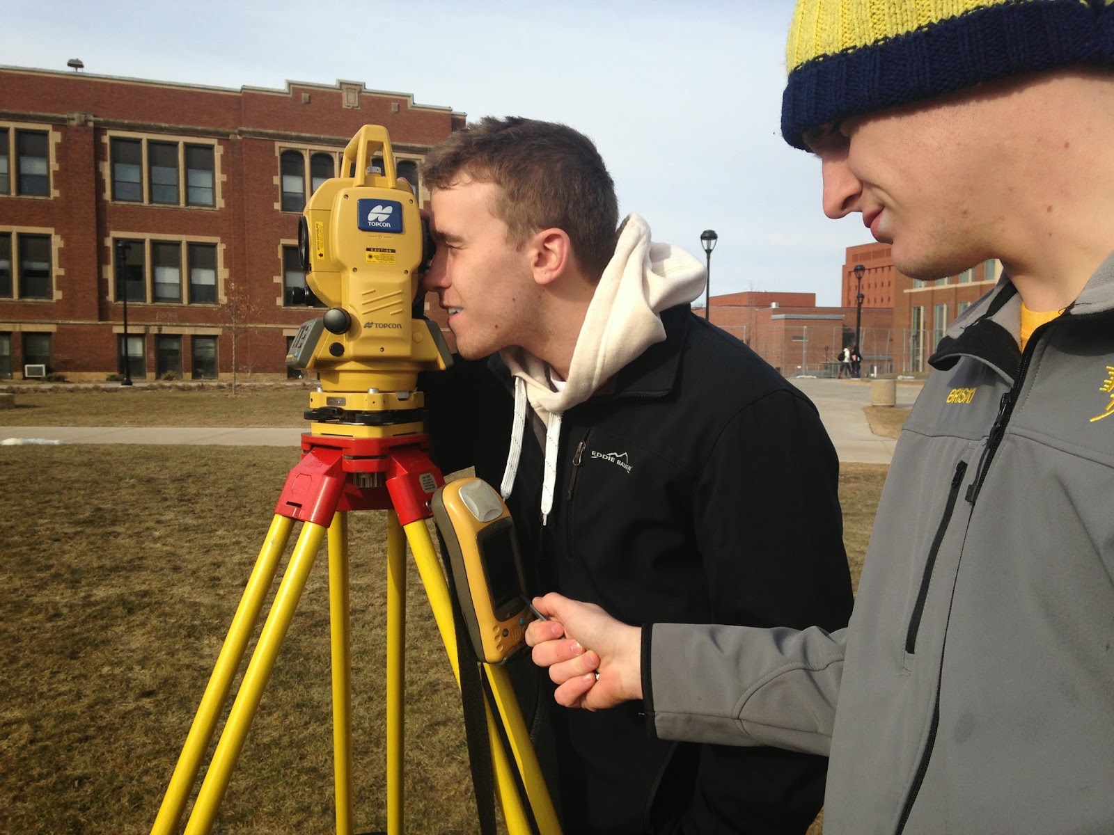
Figure 3: Image of me looking through the total station lens trying the find the prism.
Drew is ready to hit the collect button on the GPS once the total station and prism are matched.  

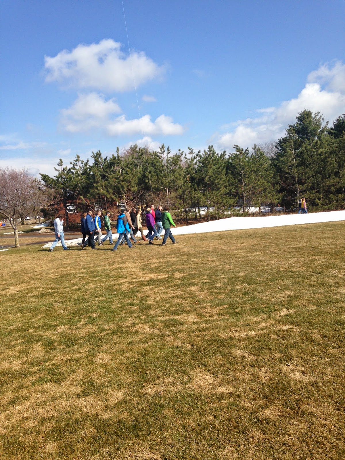
Figure 4: Image of me finding Andrew holding up the prism.  As you can see
he is about 50 meters away wearing a black shirt.  The total station has very
good optics so finding someone at a distance is easy.  

     1.      Collect Data
a.      Go to the Col menu and choose observations.
b.      Then click measure once the TSS is sighted to the prism. Continue to do this and make sure that the point’s id numbers are increasing.
c.       If you wish to verify the data, go to edit and list and look at the points you collected. You can also view these points on the map tab
d.      Continue collecting data.
e.      Be sure that if you change the height of the rod you must enter the new height of the rod into the collection screen for each point. 


After the collection is over the next step is to add the data onto ArcMap.  One problem that occured when bring the points into ArcMap was that they were flipped.  To unflip them the rotate tool was used so the points were in their correct positions.  

Results

The results of our surveying turned out well.  The amount of points that were collected worked out and gave us a good read of the elevation on campus.  However, I wish we would have surveyed more points down by the river to really see the elevation change down there.  The land surveyed was relatively flat making it easy to survey and the results don't look as cool when the land is flat.  

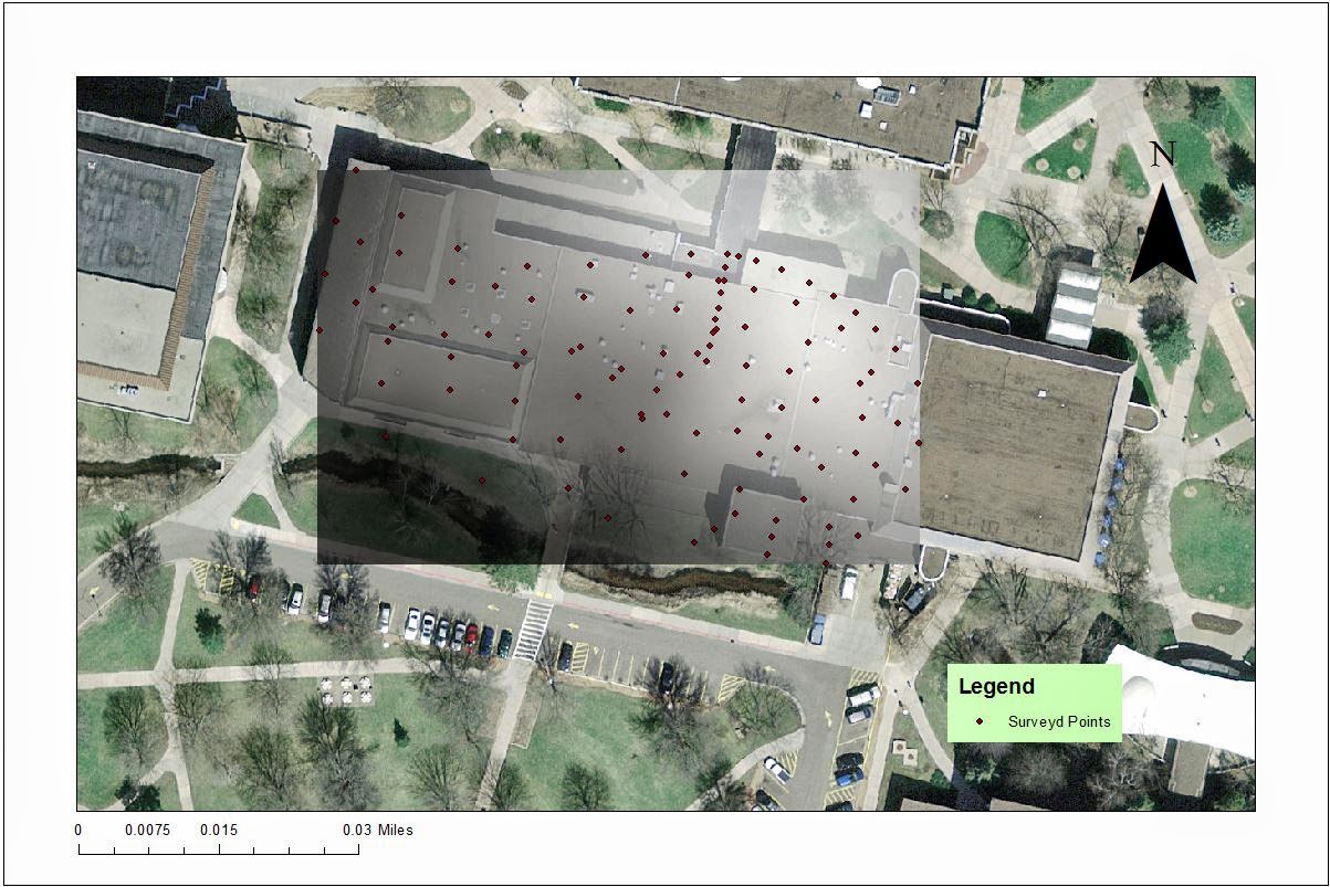
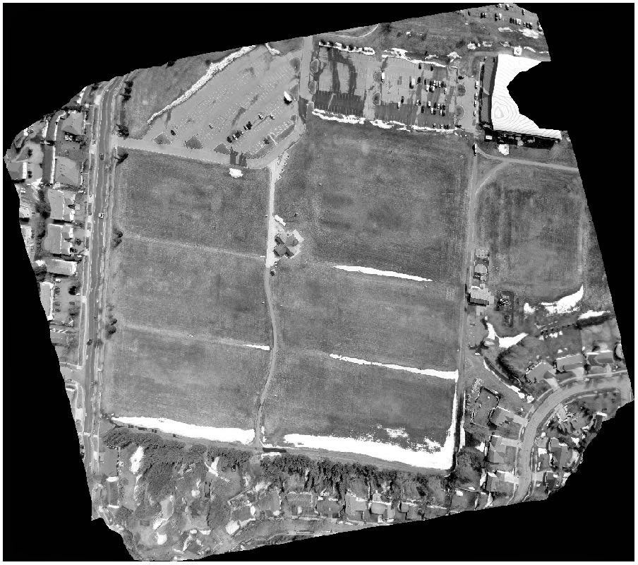
Figure 5: 2D result captured on an aerial image.  I could not find an updated image as
the building on our points does not exist anymore.
The black represents low elevation while the white is high

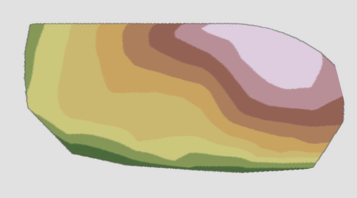
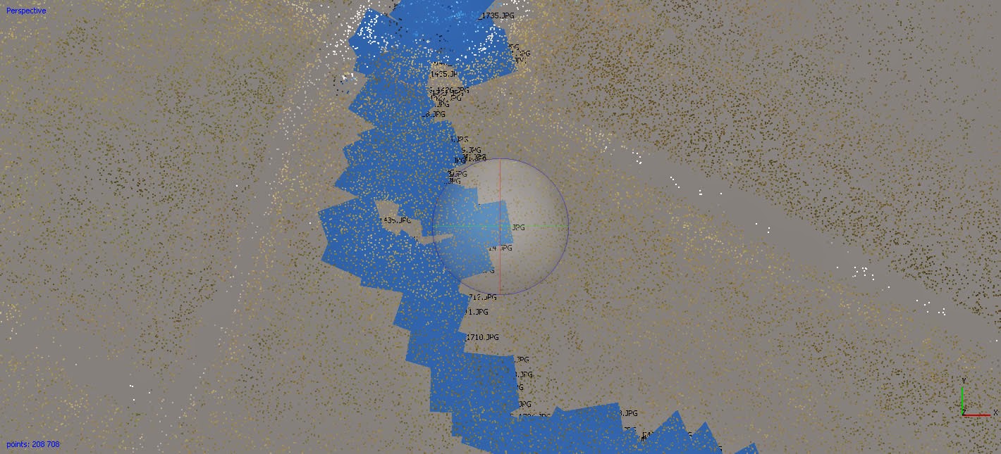
Figure 6: This is also an image of the points collected using ArcScene.
Natural neighbor was applied to the points resulting in the white being high elevation
and the green being low.  

Because of the area we surveyed and the elevation not changing much it was hard to get a 3D picture of the elevation.  When using an interpolation method in ArcScene the result would be flat, there for not being able to see a change in elevation.  


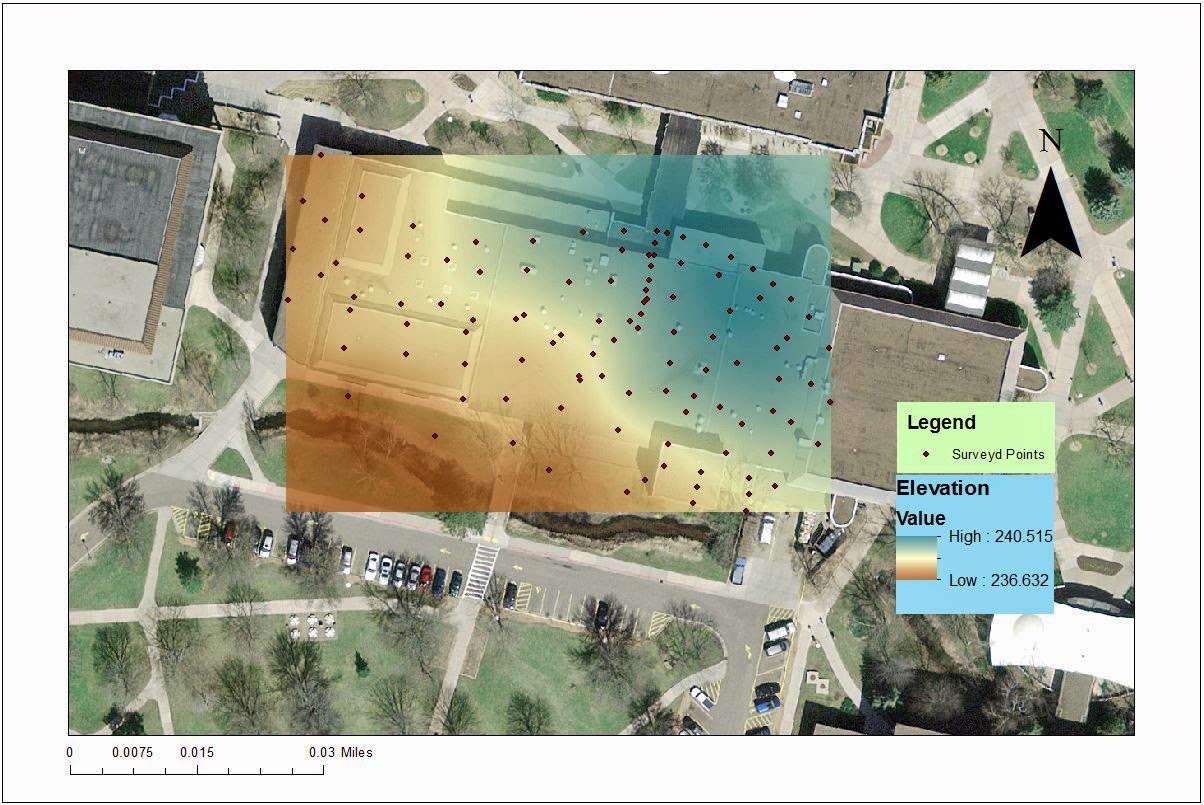
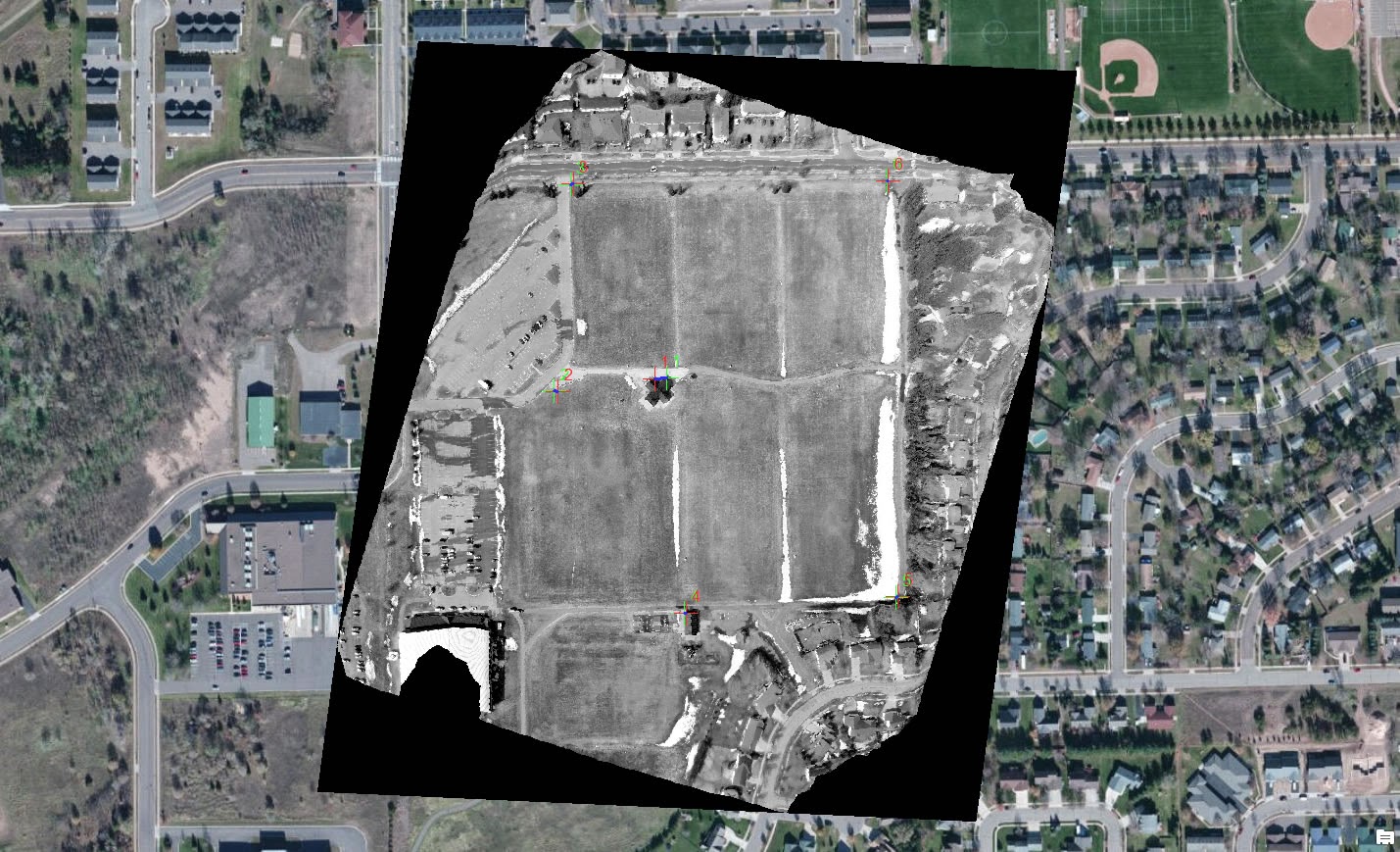
Figure 7: A final cleaner map of the points collected.  This color scheme makes it easier to read where the
low and high elevations are.


Conclusion

My group worked very well together when collecting the data.  The collection went fairly quick as I have had experience with a total station before allowing me to find the prism at a quick rate.  We had trouble setting up the GPS with switching modes to be able to collect the back sight and OCC point.  Once that was taken care of it was easy rider after that.  I would have liked to survey a place that had a greater change in elevation for a better looking 3D map and better practice when collecting an area with great elevation change.  

Sunday, March 30, 2014

Field Activity #8: ArcPad Data Collection

Introduction

This weeks activity involved gathering micro climate data using a Trimble GPS unit and temperature gauge, then mapping the information by using ArcMap.  The class was divided into groups of two and the task was to gather points in an area on the campus of University of Wisconsin Eau-Claire.  The activity called for collecting temperature, dew point, relative humidity, snow depth, wind direction, as North, South, East and West, and also azimuth 0-360 degrees, wind speed, time, and any notes to help better the collection.  After all the groups collected data for their area the points were compiled into one geodatabase ready to be used to map out the results.  

Methods

The first step of this activity is getting the GPS unit and ArcMap ready for the collection.  Two weeks ago, see field activity #6 blog, a domain was created for this assignment and was placed, along with a raster image of UWEC's campus into ArcMap.  To load the domain, or feature class, and raster image on to the GPS or ArcPad these steps need to be taken.  In ArcMap click on customize>extensions> and check ArcPad Data Manager, this will allow you to use that tool.  Next add the toolbar to ArcMap by clicking Customize>Tool bars> ArcPad Data Manager.  Then click the first button as figure 1 displays to start adding the data to the trimble unit.  

Figure 1: Click on Get Data for ArcPad
After clicking this button a box will appear and click next from the welcome screen.  Hit the action menu and choose all Geodatabase layers, and also click on the raster image and click export as background TIFF.  Then in the next screen under specify a name type 'micro_yourusername' this will create a folder for all the information.  Also change the path of where the file is stored by clicking on the little folder and put in the folder you wish to store the ArcPad data information.  Then in the next window click on create the ArcPad data on this computer and finish.  Once the project is created, copy the folder and paste it for backup in case there is an error in the process or out on the field.  

The next step is to put the new feature class and tiff image onto the ArcPad GPS unit.  Connect the trimble unit with a USB port, and once the Trimble unit is in the computer and files can be viewed copy and past the newly created folder into the storage card of the Trimble unit.  After this is done disconnect the trimble and click the button top right corner labeled ArcPad 10 as you can see in figure 2 below.  Next hit open new map and choose the new folder that created for this process, figure 3.

Figure 2: ArcPad 10

Figure 3: Choose new map to open

After these steps and with the raster image loaded to the device you are ready to go out into the field and collect data.  Using the Trimble GPS unit, figure 4, a compass, meter stick, and the Kestral device collecting the data should run quite smooth.

Figure 4: Trimble GPS unit.  When first turning on the trimble make sure the GPS is getting a signal or fix,
to allow for the GPS to know your exact location of the points created. 

Figure 5: Kestrel device, can read temperature, dew point, relative humidity, and wind speed.  

Once out in the field and in the study you and a partner can work as a team to collect the data quickly.  In trimble unit find the green circle button that collects a point and allows you to enter the information for temp, dew point, wind speed, etc.  Use the meter stick to measure snow depth, compass to find the wind azimuth and direction and the arrows on the kestrel unit will allow to move across the different elements of temperature.  Once collecting all the information move onto the next point, since this is a micro-climate activity it is wise to collect points that are relatively close to each other, about 20 or 30 yards.  

Figure 6: My partner and I study area and the 23 points we collected.  As you can see we collected
points on the eastern side of campus.  After looking at the points collected
we could have done a better job at collecting more points to gather more information. 

Figure 7: Image of UWEC's campus and the class's study area.  A total
of 268 points were collected. 
After enough points are collected the next step is to take the trimble unit back to the computer and upload the points on to ArcMap.  This is done by going back to the ArcPad Data Manager and clicking on the fourth button 'get data from ArcPad.  In the box hit the green plus arrow navigate to the new folder with points and click import graphics or check in. After this is done the new feature class containing the points with the micro climate information will appear in the geodatabase created for this activity.  The next step is to merge all of the groups information into one feature class so the information can be mapped.  The step for this can be found in Tim Condon's blog, a classmates of mine, found here.  


The next step of the activity is to create a series of map's that display the information collected.  This was done by adding the merged feature class of the all the groups.  Then using the feature class's symbology to display different types of information.  To create continuous maps of temperature, dew point, snow depth, and relative humidity the arc tool box > 3D analyst tools and the interpolation technique of natural neighbors was used to map the data.  Also one of the assignments was to create a map that showed the wind speed and direction this was done in symbology> quantities> graduated colors> advanced> rotation and rotating it by wind direction azimuth.  An arrow symbol was used to show the direction of the wind as you can see in figure 8 below.  

Results

Figure 8: Map of Wind Speed and Direction, the wind were rather calm on this day only 3 reaching
over 10 mph, also the wind direction seemed to trend as a NW wind ,coming from, making the temps colder.


Figure 9: Relative Humidity Map, increased from west to east.  

Figure 10: Snow Depth Map of the Snow depths on campus in centimeters.  The snow levels
were rather low unless some snow was shoveled or plowed making the levels higher

Figure 11: Temperature map of Eau Claire, this is an interesting map as the
only real high temps came in one circle, it could have been a group error or located near a
heater. 

Figure 12: Temperature and Relative Humidity Map, there seems to be no trend
between relative humidity and temperature.  

Figure 13: Map of temperature and wind speed + direction.
This map shows that colder temperatures are associated with higher wind speeds, which makes sense.  However there is a wind speed of 10-11 in the warmest spot which is interesting to me.  It makes me believe that there was a heater or error by the group collecting the data.  

All of the maps do a good job of representing the data collected and some patterns can be seen.  There were some errors by group 3 and points had to be deleted between Murray and Towers Hall.  Somehow the points got placed near the equator which is very strange.  These points were deleted to make the interpolation techniques work.  

Conclusion

I thought this activity was very fun to complete.  I enjoyed making the maps to find the results of all data collected and I am very happy of how my maps turned out.  I wish I would know more about weather so I can make connections and see patterns more easily.  For example, the relationship between temperature, dew point, and relative humidity and how they effect each other.  In all it was a great learning experience for the class and a skill that is going to be very useful for the future.